Traditionally, programmers are taught the basics via command line output:
1. TEXT IN → You write your code as text.
2. TEXT OUT → Your code produces text output on the command line.
3. TEXT INTERACTION → The user can enter text on the command line to interact with the program.
The output “ Hello, World! ” of this example program is an old joke, a programmer’s convention where the text output of the first program you learn to write in any given language says “ Hello, World! ” It first appeared in a 1974 Bell Laboratories memorandum by Brian Kernighan entitled “Programming in C: A Tutorial. ”
The strength of learning with Processing is its emphasis on a more intuitive and visually responsive environment, one that is more conducive to artists and designers learning programming.
1. TEXT IN → You write your code as text.
2. VISUALS OUT → Your code produces visuals in a window.
3. MOUSE INTERACTION → The user can interact with those visuals via the mouse.
Processing is not the first language to follow this paradigm. In 1967, the Logo programming language was developed by Daniel G. Bobrow, Wally Feurzeig, and Seymour Papert. With Logo, a programmer writes instructions to direct a turtle around the screen, producing shapes and designs. John Maeda’s Design By Numbers (1999) introduced computation to visual designers and artists with a simple, easy to use syntax.
Processing , a direct descendent of Logo and Design by Numbers was born in 2001 in the “ Aesthetics and Computation ” research group at the Massachusetts Institute of Technology Media Lab. It is an open source initiative by Casey Reas and Benjamin Fry, who developed Processing as graduate students studying with John Maeda.
“Processing is an open source programming language and environment for people who want to program images, animation, and sound. It is used by students, artists, designers, architects, researchers, and hobbyists for learning, prototyping, and production. It is created to teach fundamentals of computer programming within a visual context and to serve as a software sketchbook and
professional production tool. Processing is developed by artists and designers as an alternative to proprietary software tools in the same domain.”
— www.processing.org
LETS CREATE SOMETHING BIG....
There is nothing wrong with having grand visions, but the most important favor you can do for yourself is to learn how to break those visions into small parts and attack each piece slowly, one at a time. If you were to sit down and attempt to program its features all at once, I am pretty sure you would end up using a cold compress to treat your pounding headache.
When all is said and done, computer programming is all about writing algorithms . An algorithm is a sequential list of instructions that solves a particular problem. And the philosophy of incremental development (which is essentially an algorithm for you, the human being, to follow) is designed to make it easier for you to write an algorithm that implements your idea.
Try writing an algorithm for something you do on a daily basis, such as brushing your teeth. Make sure the instructions seem comically simple (as in “ Move the toothbrush one centimeter to the left ” ). Imagine that you had to provide instructions on how to
accomplish this task to someone entirely unfamiliar with toothbrushes, toothpaste, and teeth. That is how it is to write a program. A computer is nothing more than a machine that is brilliant at following precise instructions, but knows nothing about the world at large. And this is where we begin our journey, our story, our new life as a programmer. We begin with learning how to talk to our friend, the
computer.
1. TEXT IN → You write your code as text.
2. TEXT OUT → Your code produces text output on the command line.
3. TEXT INTERACTION → The user can enter text on the command line to interact with the program.
The output “ Hello, World! ” of this example program is an old joke, a programmer’s convention where the text output of the first program you learn to write in any given language says “ Hello, World! ” It first appeared in a 1974 Bell Laboratories memorandum by Brian Kernighan entitled “Programming in C: A Tutorial. ”
The strength of learning with Processing is its emphasis on a more intuitive and visually responsive environment, one that is more conducive to artists and designers learning programming.
1. TEXT IN → You write your code as text.
2. VISUALS OUT → Your code produces visuals in a window.
3. MOUSE INTERACTION → The user can interact with those visuals via the mouse.
Processing is not the first language to follow this paradigm. In 1967, the Logo programming language was developed by Daniel G. Bobrow, Wally Feurzeig, and Seymour Papert. With Logo, a programmer writes instructions to direct a turtle around the screen, producing shapes and designs. John Maeda’s Design By Numbers (1999) introduced computation to visual designers and artists with a simple, easy to use syntax.
Processing , a direct descendent of Logo and Design by Numbers was born in 2001 in the “ Aesthetics and Computation ” research group at the Massachusetts Institute of Technology Media Lab. It is an open source initiative by Casey Reas and Benjamin Fry, who developed Processing as graduate students studying with John Maeda.
“Processing is an open source programming language and environment for people who want to program images, animation, and sound. It is used by students, artists, designers, architects, researchers, and hobbyists for learning, prototyping, and production. It is created to teach fundamentals of computer programming within a visual context and to serve as a software sketchbook and
professional production tool. Processing is developed by artists and designers as an alternative to proprietary software tools in the same domain.”
— www.processing.org
LETS CREATE SOMETHING BIG....
There is nothing wrong with having grand visions, but the most important favor you can do for yourself is to learn how to break those visions into small parts and attack each piece slowly, one at a time. If you were to sit down and attempt to program its features all at once, I am pretty sure you would end up using a cold compress to treat your pounding headache.
When all is said and done, computer programming is all about writing algorithms . An algorithm is a sequential list of instructions that solves a particular problem. And the philosophy of incremental development (which is essentially an algorithm for you, the human being, to follow) is designed to make it easier for you to write an algorithm that implements your idea.
Try writing an algorithm for something you do on a daily basis, such as brushing your teeth. Make sure the instructions seem comically simple (as in “ Move the toothbrush one centimeter to the left ” ). Imagine that you had to provide instructions on how to
accomplish this task to someone entirely unfamiliar with toothbrushes, toothpaste, and teeth. That is how it is to write a program. A computer is nothing more than a machine that is brilliant at following precise instructions, but knows nothing about the world at large. And this is where we begin our journey, our story, our new life as a programmer. We begin with learning how to talk to our friend, the
computer.
|
Open up a processing file and simply type in
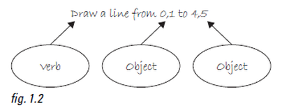
line(1,0,4,5); Congratulations, you have written your first line of computer code! We will get to the precise formatting of the above later, but for now, even without knowing too much, it should make a fair amount of sense. We are providing a command (which we will refer to as a “ function ” ) for the machine to follow entitled“ line. ” In addition, we are specifying some arguments for how that line should be drawn, from point A (0,1) to point B (4,5). If you think of that line of code as a sentence, the function is a verb and the arguments are the objects of the sentence. The code sentence also ends with a semicolon instead of a period. |
|
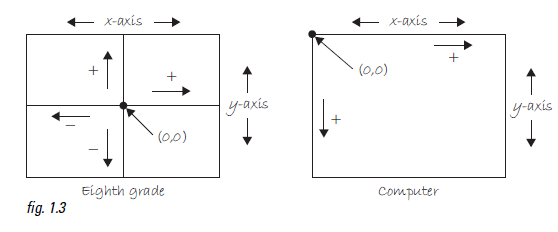
The key here is to realize that the computer screen is nothing more than a fancier piece of graph paper. Each pixel of the screen is a coordinate—two numbers, an “x ” (horizontal) and a “ y ” (vertical)—that determine the location of a point in space. And it is our job to specify what shapes and colors should appear at these pixel coordinates.
Nevertheless, there is a catch here. The graph paper from eighth grade ( “ Cartesian coordinate system ” ) placed (0,0) in the center with the y-axis pointing up and the x-axis pointing to the right (in the positive direction, negative down and to the left). The coordinate
system for pixels in a computer window, however, is reversed along the y -axis. (0,0) can be found at the top left with the positive direction to the right horizontally and down vertically. See Figure 1.3 .
Try it out!, Make sure you make a new "line" with each code, and end each line with a semicolon.
1.2 Simple Shapes
The vast majority of the programming examples in this book will be visual in nature. You may ultimately learn to develop interactive games, algorithmic art pieces, animated logo designs, and (insert your own category here) with Processing, but at its core, each visual program will involve setting pixels. The simplest way to get started in understanding how this works is to learn to draw primitive shapes. This is not unlike how we learn to draw in elementary school, only here we do so with code instead of crayons.
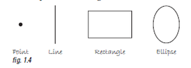
Let’s start with the four primitive shapes shown in Figure 1.4
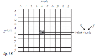
For each shape, we will ask ourselves what information is required to specify the location and size (and later color) of that shape and learn how Processing expects to receive that information. In each of the diagrams below ( Figures 1.5 through 1.11), assume a window with a width of 10 pixels and height of 10 pixels. This isn’t particularly realistic since when we really start coding we will most likely work with much larger windows (10 x10 pixels is barely a few millimeters of screen space). Nevertheless for demonstration purposes, it is nice to work with smaller numbers in order to present the pixels as they might appear on graph paper (for now) to better illustrate the inner workings of each line of code.
|
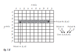
A point is the easiest of the shapes and a good place to start. To draw a point, we only need an x and y coordinate as shown in Figure 1.5 . A line isn’t terribly difficult either. A line requires two points, as shown in Figure 1.6 .
point(4,5); line(1,3,8,3); |
|
|
|
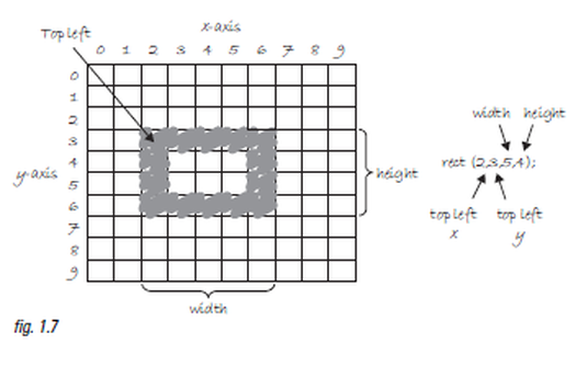
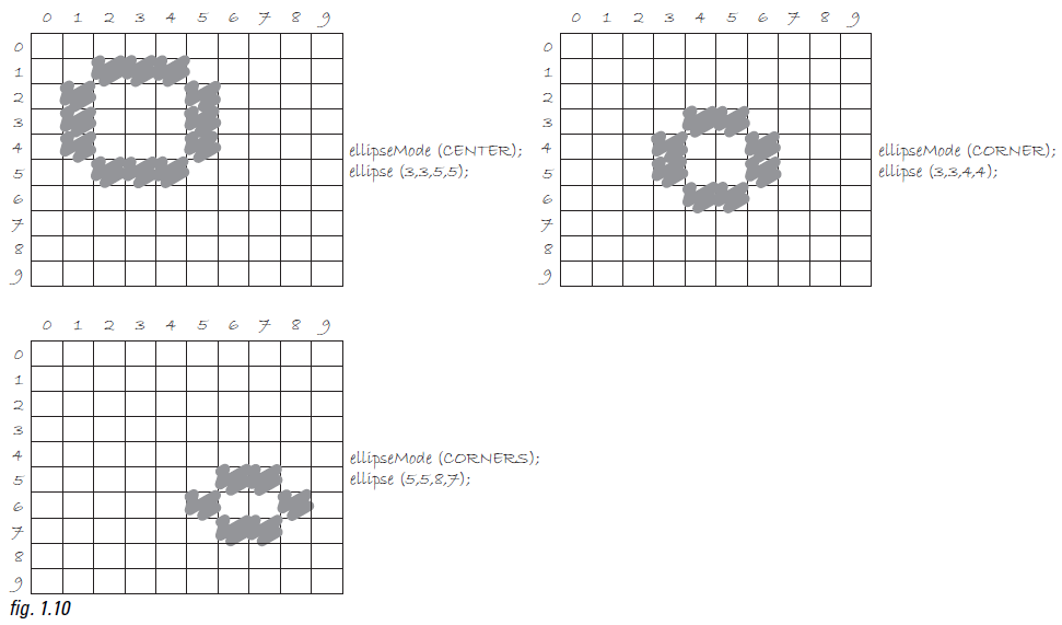
Once we arrive at drawing a rectangle, things become a bit more complicated. In Processing , a rectangle is specified by the coordinate for the top left corner of the rectangle, as well as its width and height (see Figure 1.7 ).
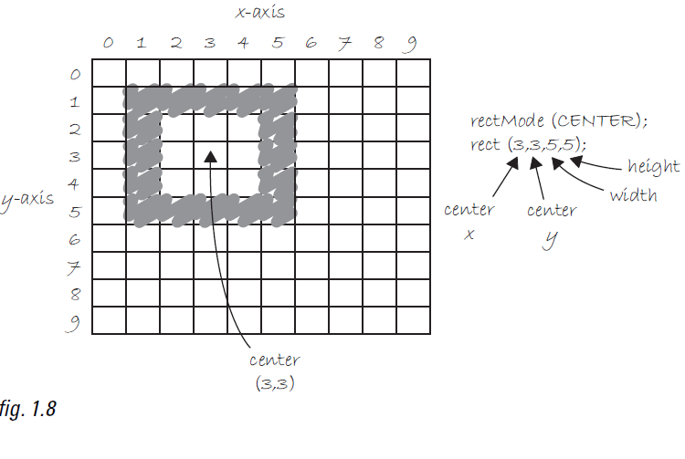
rect(2,3,5,4); However, a second way to draw a rectangle involves specifying the centerpoint, along with width and height as shown in Figure 1.8 . If we prefer this method, we first indicate that we want to use the “ CENTER ” mode before the instruction for the rectangle itself. Note that Processing is
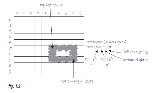
case-sensitive. Incidentally, the default mode is “ CORNER, ” which is how we began as illustrated in Figure 1.7 . Finally, we can also draw a rectangle with two points (the top left corner and the bottom right corner). The mode here is “ CORNERS ” (see Figure 1.9) Once we have become comfortable with the concept of drawing a rectangle, an ellipse is a snap. In fact, it is identical to rect( ) with the difference being that an ellipse is drawn where the bounding box 1 of the rectangle would be. The default mode for ellipse( ) is “ CENTER ” , rather than “ CORNER ” as with rect( ) |
|
|
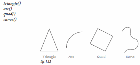
Certainly, point, line, ellipse, and rectangle are not the only shapes available in the Processing library of functions. In Chapter 2, we will see how the Processing reference provides us with a full list of available drawing functions along with documentation of the
required arguments, sample syntax, and imagery. For now, as an exercise, you might try to imagine what arguments are required for some other shapes (Figure 1.12): . |
|
1.3 Grayscale Color
The primary building block for placing shapes onscreen is a pixel coordinate. You politely instructed the computer to draw a shape
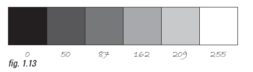
at a specific location with a specific size. Nevertheless, a fundamental element was missing—color. In the digital world, precision is required. Saying “ Hey, can you make that circle bluish-green? ” will not do. Therefore, color is defined with a range of numbers. Let’s start with the simplest case: black and white or grayscale . In grayscale terms, we have the following: 0 means black, 255 means white. In between, every other number—50, 87, 162, 209, and so on—is a shade of gray ranging from black to white. See
Figure 1.13 .
The primary building block for placing shapes onscreen is a pixel coordinate. You politely instructed the computer to draw a shape
at a specific location with a specific size. Nevertheless, a fundamental element was missing—color. In the digital world, precision is required. Saying “ Hey, can you make that circle bluish-green? ” will not do. Therefore, color is defined with a range of numbers. Let’s start with the simplest case: black and white or grayscale . In grayscale terms, we have the following: 0 means black, 255 means white. In between, every other number—50, 87, 162, 209, and so on—is a shade of gray ranging from black to white. See
Figure 1.13 .
Have you seen 0-255 before??
Understanding how this range works, we can now move to setting specific grayscale colors for the shapes we drew before. In Processing, every shape has a stroke( ) or a fill( ) or both. The stroke( ) is the outline of the shape, and the fill( ) is the interior of that shape. Lines and points can only have stroke( ) , for obvious reasons. If we forget to specify a color, Processing will use black (0) for the stroke( ) and white (255) for the fill( ) by default.
Understanding how this range works, we can now move to setting specific grayscale colors for the shapes we drew before. In Processing, every shape has a stroke( ) or a fill( ) or both. The stroke( ) is the outline of the shape, and the fill( ) is the interior of that shape. Lines and points can only have stroke( ) , for obvious reasons. If we forget to specify a color, Processing will use black (0) for the stroke( ) and white (255) for the fill( ) by default.
|
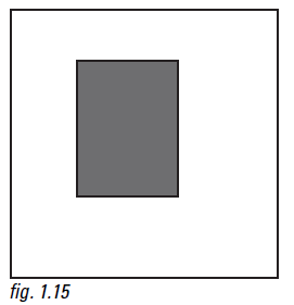
Here is an example of
rect(50,40,75,100); |
|
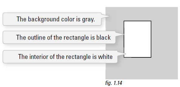
By adding the stroke( ) and fill( ) functions before the shape is drawn, we can set the color. It is much like instructing your friend to use a specific pen to draw on the graph paper. You would have to tell your friend before he or she starting drawing, not after. There is also the function background( ), which sets a background color for the window where shapes will be rendered.
|
background(255);
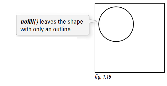
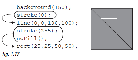
stroke(0); fill(150); rect(50,50,75,100); stroke( ) or fill( ) can be eliminated with the noStroke( ) or noFill( ) functions. Our instinct might be to say “stroke(0)” for no outline, however, it is important to remember that 0 is not “ nothing ” , but rather denotes the color black. Also, remember not to eliminate both—with noStroke( ) and noFill( ), nothing will appear! Another example: background(255); stroke(0); noFill(); ellipse(60,60,100,100); If we draw two shapes at one time, Processing will always use the most recently specified stroke( ) and fill( ), reading the code from top to bottom.
|
|
Task:
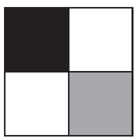
Create, and test, the code which would produce the following:
Start with rect(0,0,50,50);
Create, and test, the code which would produce the following:
Start with rect(0,0,50,50);
Other various simple codes:
size(320,240); - Makes the window 320 wide and 240 tall.
println( ) - takes one argument, a String of characters enclosed in quotes, and produces it in the Processing Window.
// - Comments Example:
// This is a comment on one line
/* Th is is a comment that
spans several lines
of code */
Task:
Each line below has an error in it, fix it and run the correct program..
size(200,200)
background();
stroke 255;
fill (150)
rectMode (center);
rect (100,100,50);
1.4 RGB Color
A nostalgic look back at graph paper helped us learn the fundamentals for pixel locations and size. Now that it is time to study the basics of digital color, we search for another childhood memory to get us started. Remember finger painting? By mixing three “primary ” colors, any color could be generated. Swirling all colors together resulted in a muddy brown. The more paint you added, the darker it got. Digital colors are also constructed by mixing three primary colors, but it works differently from paint.
First, the primaries are different: red, green, and blue (i.e., “ RGB ” color). And with color on the screen, you are mixing light, not paint, so the mixing rules are different as well.
• Red+green=yellow
• Red+blue= purple
• Green+blue=cyan (blue-green)
• Red+green+blue=white
• No colors =black
This assumes that the colors are all as bright as possible, but of course, you have a range of color available, so some red plus some green plus some blue equals gray, and a bit of red plus a bit of blue equals dark purple. While this may take some getting used to, the more you program and experiment with RGB color, the more it will become instinctive, much like swirling colors with your
fingers. And of course you can’t say “ Mixsome red with a bit of blue, ” you have to provide an exact amount. As with grayscale, the individual color elements are expressed as ranges from 0 (none of that color) to 255 (as much as possible), and they are listed
in the order R, G, and B. You will get the hang of RGB color mixing through experimentation, but next we will cover some code using some common colors.
|
Example:
background(255); noStroke(); fill(255,0,0); ellipse(20,20,16,16); fill(127,0,0); ellipse(40,20,16,16); fill(255,200,200); ellipse(60,20,16,16); |

|
Processing also has a color selector to aid in choosing colors. Access this via TOOLS (from the menu bar) → COLOR SELECTOR.
Task:
Change the code above to create three drastically different colors, and create a comment for what each color is.
1.5 Color Transparency
In addition to the red, green, and blue components of each color, there is an additional optional fourth component, referred to as the color’s “ alpha. ” Alpha means transparency and is particularly useful when you want to draw elements that appear partially see-through on top of one another. The alpha values for an image are sometimes referred to collectively as the “ alpha channel ” of an image. It is important to realize that pixels are not literally transparent, this is simply a convenient illusion that is accomplished by blending colors. Behind the scenes, Processing takes the color numbers and adds a percentage of one to a percentage of another, creating the optical perception of blending. (If you are interested in programming “ rose-colored ” glasses, this is where you would begin.)
Alpha values also range from 0 to 255, with 0 being completely transparent (i.e., 0% opaque) and 255 completely opaque (i.e., 100% opaque).
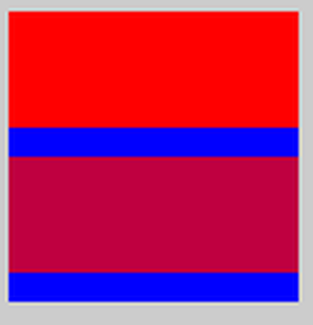
|
background(0);
noStroke( ); fill(0,0,255); rect(0,0,100,200); fill(255,0,0,255); rect(0,0,200,40); fill(255,0,0,191); rect(0,50,200,40); fill(255,0,0,127); rect(0,100,200,40); fill(255,0,0,63); rect(0,150,200,40); |
|
1.6 Custom Color Ranges
RGB color with ranges of 0 to 255 is not the only way you can handle color in Processing . Behind the scenes in the computer’s memory, color is always talked about as a series of 24 bits (or 32 in the case of colors with an alpha). However, Processing will let us think about color any way we like, and translate our values into numbers the computer understands. For example, you might prefer to think of color as ranging from 0 to 100 (like a percentage). You can do this by specifying a custom colorMode( ) .
Example:
colorMode(RGB,100); //This puts the mode into RBG and only 0-100 values.
Although it is rarely convenient to do so, you can also have different ranges for each color component:
colorMode(RGB,100,500,10,255); //Red values go from 0 to 100, green from 0 to 500, blue from 0 to 10, and alpha from 0 to 255.
Finally, while you will likely only need RGB color for all of your programming needs, you can also specify colors in the HSB (hue, saturation, and brightness) mode. Without getting into too much detail, HSB color works as follows:
• Hue —The color type, ranges from 0 to 360 by default (think of 360° on a color “ wheel ” ).
• Saturation —The vibrancy of the color, 0 to 100 by default.
• Brightness —The, well, brightness of the color, 0 to 100 by default.
TEXT:
To learn how to input text please click and read
https://www.processing.org/reference/text_.html
TASK: Create a program that creates what you see below
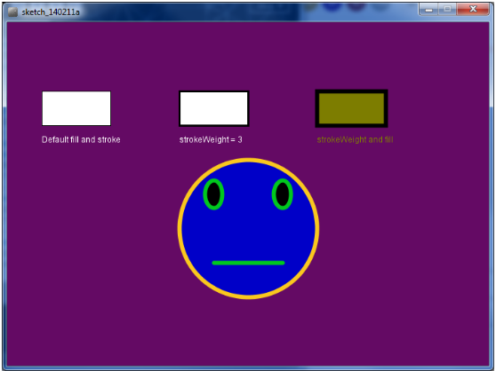
Step 1: Begin with the following code:
size(700, 500);
Step 2: Draw three equally sized rectangles across the screen
Step 3: Label the rectangles with text to match the example
Step 4: Change the stroke, strokeWeight and fill colours for each rectangle
Step 5: Draw a large circle, centred on the screen. Change the stroke, strokeWeight and fill colours as you wish.
Step 6: Draw two eyes. Change the stroke, strokeWeight and fill colours as you wish.
Step 7: Draw the mouth. Change the stroke, strokeWeight and fill colours as you wish.
HOW TO DO TEXT?
textAlign(CENTER);
text( " This text is centered. " ,width/2,60);
textAlign (LEFT) ;
text( " This text is left aligned. " ,width/2,100);
textAlign(RIGHT);
text( " This text is right aligned. " ,width/2,140);
size(700, 500);
Step 2: Draw three equally sized rectangles across the screen
- line them up evenly (same Y coordinates)
- spread them out so they are equally spaced
Step 3: Label the rectangles with text to match the example
Step 4: Change the stroke, strokeWeight and fill colours for each rectangle
Step 5: Draw a large circle, centred on the screen. Change the stroke, strokeWeight and fill colours as you wish.
Step 6: Draw two eyes. Change the stroke, strokeWeight and fill colours as you wish.
Step 7: Draw the mouth. Change the stroke, strokeWeight and fill colours as you wish.
HOW TO DO TEXT?
textAlign(CENTER);
text( " This text is centered. " ,width/2,60);
textAlign (LEFT) ;
text( " This text is left aligned. " ,width/2,100);
textAlign(RIGHT);
text( " This text is right aligned. " ,width/2,140);
